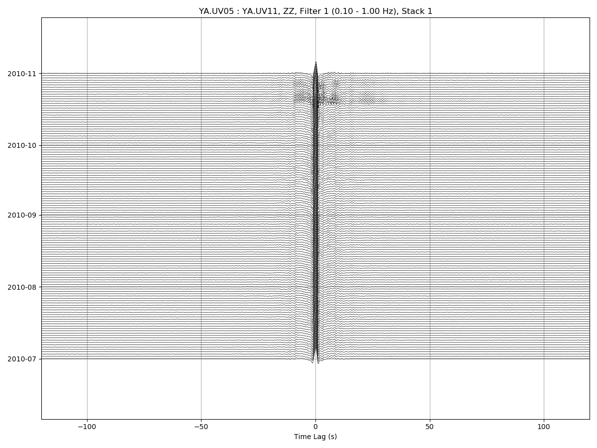
→ Plot CCF vs Time
This plot shows the cross-correlation functions (CCF) vs time. The parameters .. include:: /clickhelp/msnoise-cc-plot-ccftime.rst
allow to plot the daily or the mov-stacked CCF. Filters and components are
selectable too. The --ampli argument allows to increase the vertical scale
of the CCFs. The --seismic shows the up-going wiggles with a black-filled
background (very heavy !). Passing --refilter allows to bandpass filter
CCFs before plotting .
Example:
msnoise cc plot ccftime YA.UV06 YA.UV11 will plot all defaults:
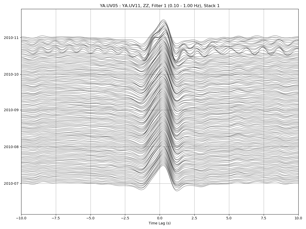
For zooming in the CCFs:
msnoise cc plot ccftime YA.UV05 YA.UV11 --xlim=-10,10 --ampli=15:
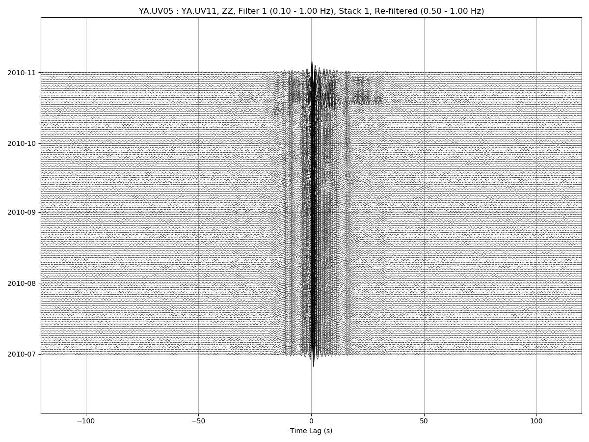
It is sometimes useful to refilter the CCFs on the fly:
msnoise cc plot ccftime YA.UV05 YA.UV11 -r 0.5:1.0:
→ Plot Interferograms
This plot shows the cross-correlation functions (CCF) vs time in a very similar .. include:: /clickhelp/msnoise-cc-plot-interferogram.rst
manner as on the ccftime plot above, but shows an image instead of wiggles.
The parameters allow to plot the daily or the mov-stacked CCF. Filters and
components are selectable too. Passing --refilter allows to bandpass filter
CCFs before plotting .
Example:
msnoise cc plot interferogram YA.UV06 YA.UV11 -m5 will plot the ZZ component
(default), filter 1 (default) and mov_stack 5:
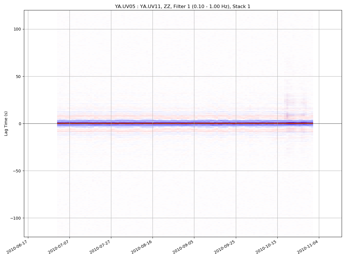
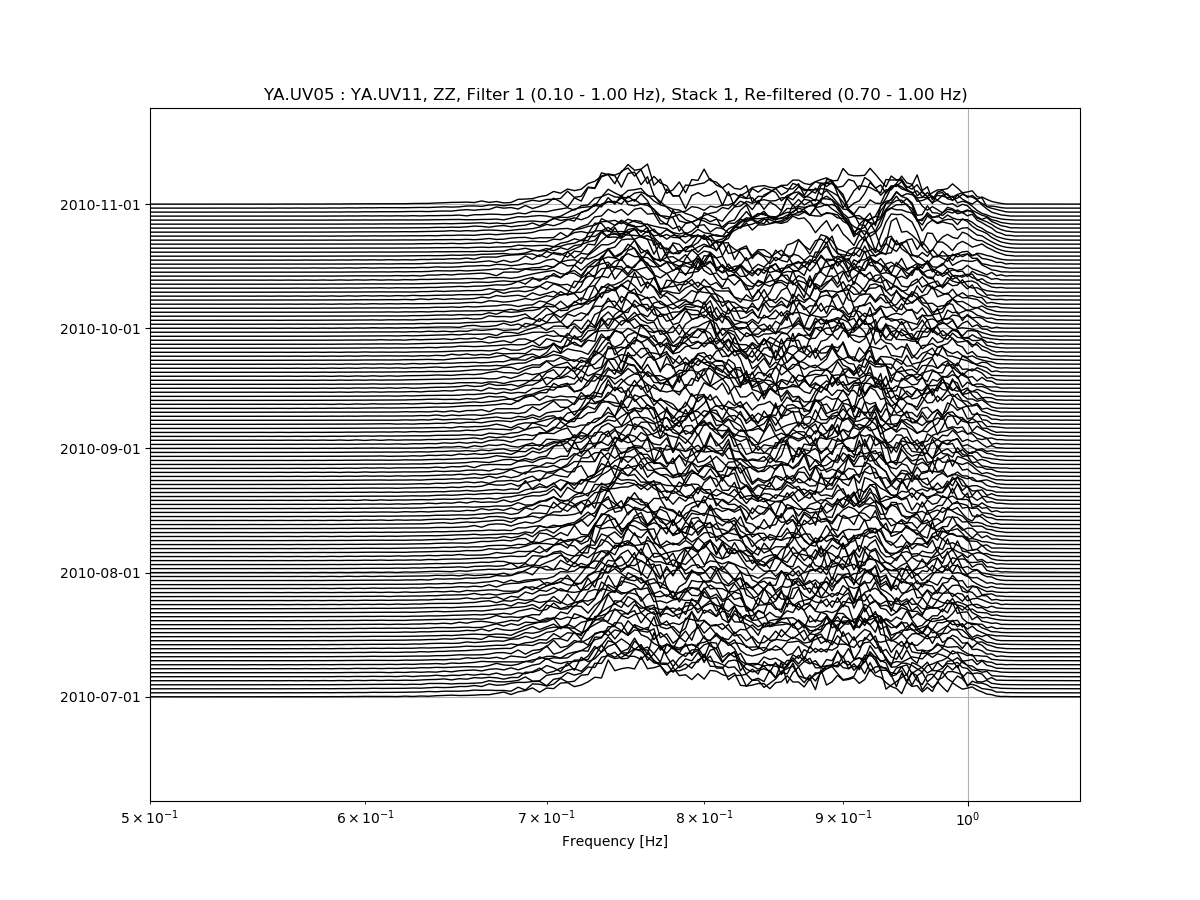
→ Plot CCF’s spectrum vs Time
This plot shows the cross-correlation functions’ spectrum vs time. The .. include:: /clickhelp/msnoise-cc-plot-spectime.rst
parameters allow to plot the daily or the mov-stacked CCF. Filters and
components are selectable too. The --ampli argument allows to increase the
vertical scale of the CCFs. Passing --refilter allows to bandpass filter
CCFs before computing the FFT and plotting. Passing --startdate and
--enddate parameters allows to specify which period of data should be
plotted. By default the plot uses dates determined in database.
Example:
msnoise cc plot spectime YA.UV05 YA.UV11 will plot all defaults:
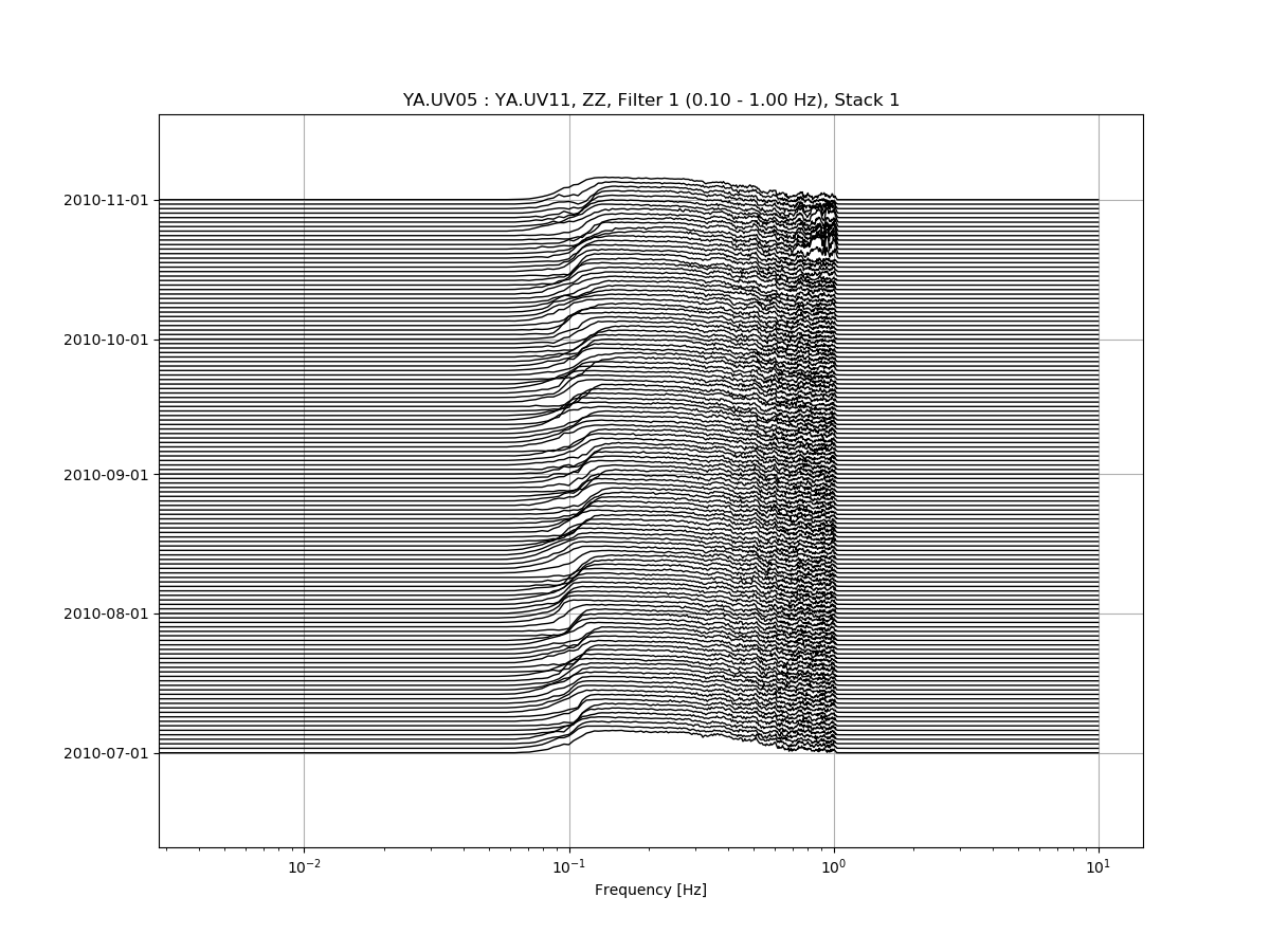
Zooming in the X-axis and playing with the amplitude:
msnoise cc plot spectime YA.UV05 YA.UV11 --xlim=0.08,1.1 --ampli=10:
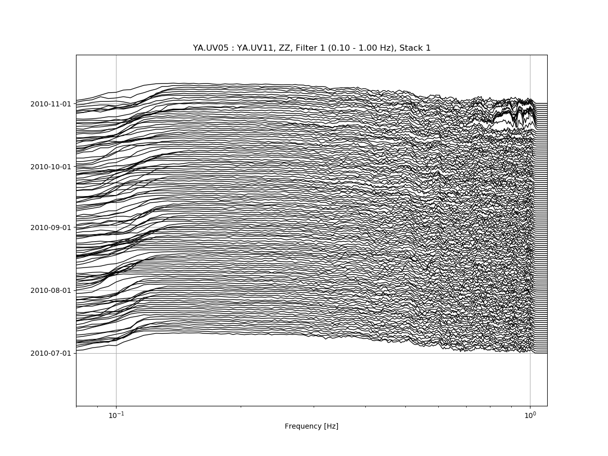
And refiltering to enhance high frequency content:
msnoise cc plot spectime YA.UV05 YA.UV11 --xlim=0.5,1.1 --ampli=10 -r0.7:1.0: