Plotting

MSNoise comes with some default plotting tools.

All plotting commands accept the --outfile argument. If provided, the figure will be saved to the disk. Names can be explicit, or tell the code to generate the filename automatically (using the ? question mark), for example:

# automatic naming, save to PNG
msnoise plot dvv -o ?.png

# automatic naming, save to PDF
msnoise plot dvv -o ?.pdf

# explicit naming, save to JPG
msnoise plot dvv -o mydvv.jpg

Customizing Plots 

All plots commands can be overridden using a -c argument in front of the plot command !!

Examples:

msnoise -c plot distance
msnoise -c plot ccftime YA.UV02 YA.UV06 -m 5
etc.

To make this work, one has to copy the plot script from the msnoise install directory to the project directory (where your db.ini file is located, then edit it to one’s desires. The first thing to edit in the code is the import of the MSNoise API:

from ..api import *

to

from msnoise.api import *

and it should work.

New in version 1.4.

Data Availability Plot 

Plots the data availability, as contained in the database. Every day which has a least some data will be coloured in red. Days with no data remain blank.

Example:

msnoise plot data_availability :

Station Map 

This plots a very raw station map (needs improvement). This plot requires cartopy !

Example:

msnoise plot station_map :

It will also generate a HTML file showing the stations on the Leaflet Mapping Service:

New in version 1.4: | Thanks to A. Mordret!

Interferogram Plot 

This plot shows the cross-correlation functions (CCF) vs time in a very similar manner as on the ccftime plot above, but shows an image instead of wiggles. The parameters allow to plot the daily or the mov-stacked CCF. Filters and components are selectable too. Passing --refilter allows to bandpass filter CCFs before plotting (new in 1.5).

Example:

msnoise cc plot interferogram YA.UV06 YA.UV11 -m5 will plot the ZZ component (default), filter 1 (default) and mov_stack 5:

CCF vs Time 

This plot shows the cross-correlation functions (CCF) vs time. The parameters allow to plot the daily or the mov-stacked CCF. Filters and components are selectable too. The --ampli argument allows to increase the vertical scale of the CCFs. The --seismic shows the up-going wiggles with a black-filled background (very heavy !). Passing --refilter allows to bandpass filter CCFs before plotting (new in 1.5).

Example:

msnoise cc plot ccftime YA.UV06 YA.UV11 will plot all defaults:

For zooming in the CCFs:

msnoise cc plot ccftime YA.UV05 YA.UV11 --xlim=-10,10 --ampli=15:

It is sometimes useful to refilter the CCFs on the fly:

msnoise cc plot ccftime YA.UV05 YA.UV11 -r 0.5:1.0:

CCF’s spectrum vs Time 

This plot shows the cross-correlation functions’ spectrum vs time. The parameters allow to plot the daily or the mov-stacked CCF. Filters and components are selectable too. The --ampli argument allows to increase the vertical scale of the CCFs. Passing --refilter allows to bandpass filter CCFs before computing the FFT and plotting. Passing --startdate and --enddate parameters allows to specify which period of data should be plotted. By default the plot uses dates determined in database.

Example:

msnoise cc plot spectime YA.UV05 YA.UV11 will plot all defaults:

Zooming in the X-axis and playing with the amplitude:

msnoise cc plot spectime YA.UV05 YA.UV11 --xlim=0.08,1.1 --ampli=10:

And refiltering to enhance high frequency content:

msnoise cc plot spectime YA.UV05 YA.UV11 --xlim=0.5,1.1 --ampli=10 -r0.7:1.0:

MWCS Plot 

This plot shows the result of the MWCS calculations in two superposed images. One is the dt calculated vs time lag and the other one is the coherence. The image is constructed by horizontally stacking the MWCS of different days. The two right panels show the mean and standard deviation per time lag of the whole image. The selected time lags for the dt/t calculation are presented with green horizontal lines, and the minimum coherence or the maximum dt are in red.

The filterid, comp and mov_stack allow filtering the data used.

Example:

msnoise cc dvv plot mwcs ID.KWUI ID.POSI -m 3 will plot all defaults with the mov_stack = 3:

Distance Plot 

Plots the REF stacks vs interstation distance. This could help deciding which parameters to use in the dt/t calculation step. Passing --refilter allows to bandpass filter CCFs before plotting (new in 1.5). It is also possible to only draw CCFs for pairs including one station by passing --virtual-pair followed by the desired NET.STA (new in 1.5).

Example:

msnoise cc plot distance will plot all defaults:

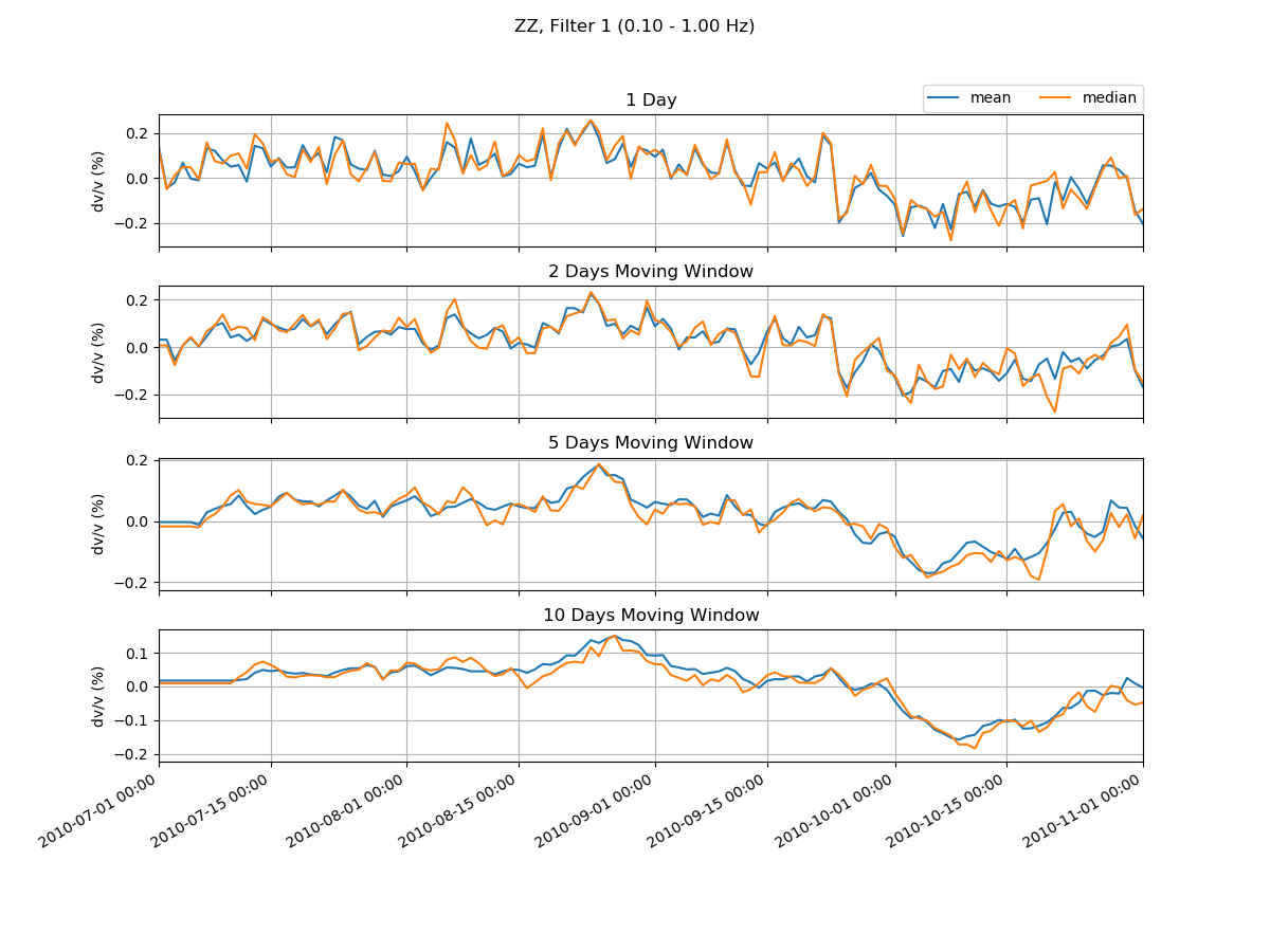
dv/v Plot 

This plot shows the final output of MSNoise.

Example:

msnoise cc dvv plot dvv will plot all defaults:

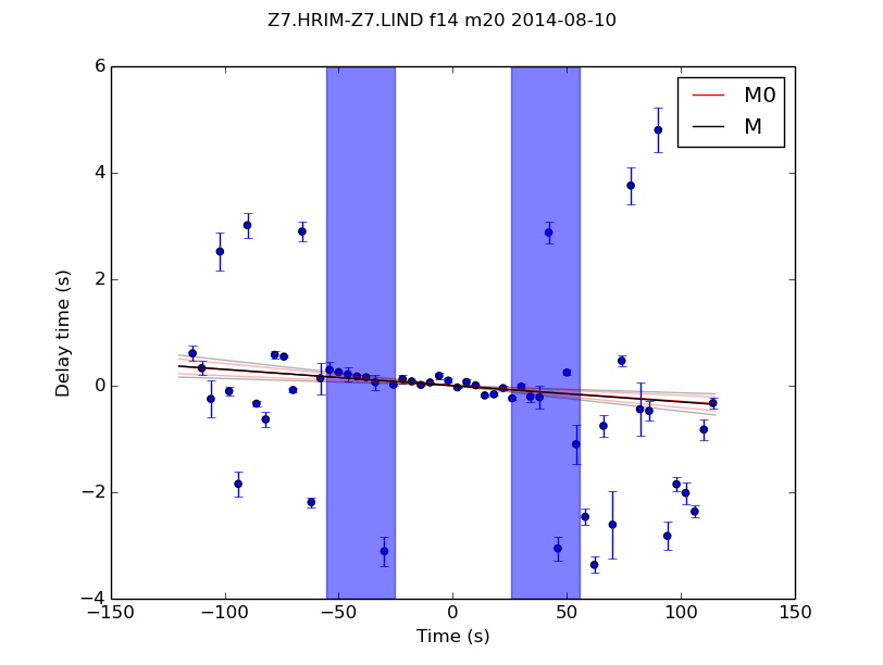
dt/t Plot 

This plots dt (delay time) against t (time lag). It shows the results from the MWCS step, plus the calculated regression lines M0 and M. The errors in the regression lines are also plotted as fainter lines. The time lags used to calculate the regression are shown in blue.

Example

msnoise cc dvv plot dtt Z7.HRIM Z7.LIND 2014-08-10 -f 14 -m 20 will plot:

New in version 1.4: (Thanks to C.G. Donaldson)